Central Limit Theorem

The central limit theorem, in layman’s terms, says that regardless of the shape of the distribution of a population, in most cases, the mean of random samples taken from that population will approximate a normal distribution. The larger the sample, or the larger the number of samples, the closer the resulting distribution will be to normal.

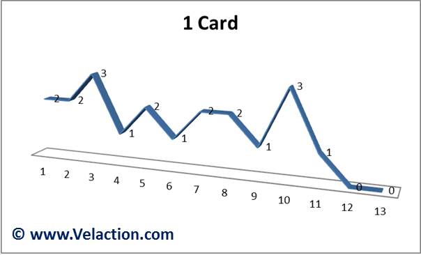
It is probably easiest to explain this concept using a deck of cards. If you assign a value of 1 to 13 to each card, and draw a single card at a time (and return it to the deck), the distribution would be flat, and a random sample of 20 cards might look something like this:

But what happens when you draw 20 hands of 5 cards each and average out the results?

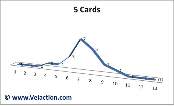
The results start to cluster around the expected average value, 7, of the entire deck.

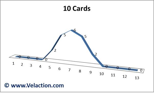
The effect gets even more pronounced as you use increasingly larger sample sizes. With 20 hands of 10 cards, the distribution is even more clearly normal. I’d like to point out that these charts are the result of a real-life card-dealing data collection effort.

You’d also get a more pronounced normal distribution as the number of samples increases. That means that 100 hands of 5 cards each will look more normal than the picture above.

Remember, the distribution curve for a deck of cards is completely flat, but the resulting distribution of the averages assumes a normal distribution curve.

Note that this effect would still be seen regardless of the shape of the underlying distribution, as long as its shape is well-defined. If you took out all the red cards above 8, you’d be skewing the population. But you’d still get a normal distribution with the same dealing/data collection process, albeit centered at a different location.

That really means that the level of variation has to be consistent. But, if you change the underlying process during a data collection effort, you change the output and the central limit theorem won’t apply. You’d shift the data. Think about what would happen if you took all the face cards out of a deck after you’ve dealt half the hands. You’d expect a shift in the look of the curves, so a mix of before and after samples would not be normal.

In practice, you might be looking at the cycle time of a process. You’d probably have a skewed distribution. Imagine you had a 10-minute average for a process. You’d be unlikely to have many times below 7 or 8 minutes, even if everything went perfect. But you could have some times in the mid-to-high teens, and maybe even an occasional 20 minute cycle if things got really crazy.

If you took a sample of each day’s cycle times and averaged them out, though, the resulting distribution would be normal. This is the basis of SPC. If there is a shift in the process, the shape of the average distribution shifts, allowing you to pick up on subtle changes.

Application of the Central Limit Theorem

SPC, or statistical process control relies on the central limit theorem. Think back to what happens if you pull out all those face cards. You’d expect a shift in the output.

SPC looks for that shift. Actually, it looks for even more subtle shifts. It can detect the removal of just a few cards as it shifts the data away from its historical standard deviation.